Unit 5 Orbits and Scattering

W. G. Harter

Whether one looks outward to the planetary, galactic, or extra-galactic heavens, or else inward to molecules, atoms, or nuclei, it all seems glued by orbits and scattering trajectories. For planets and atoms it is Coulomb orbits first quantified by Kepler, Newton, Rutherford, Bohr, and Sommerfeld. Orbitals of galaxies or electrons in solids are less clear but classical models are based on oscillator trajectories, often chaotic ones. This unit is mainly about 3D Coulomb orbit mechanics and geometry with some comparison to harmonic oscillator dynamics introduced in preceding units 1-4. A discussion of Coulomb-plus-uniform field and 2-Coulomb-center molecular orbits is also introduced.

Hyperbolic Rutherford scattering orbits envelop parabolic shadow caustic

___________________________________________________________________________________

Hamilton-Laplace-Runge-Lenz eccentricity vector e and angular momentum L geometry

Unit 5. Orbits and Scattering.......................................................................... 4

5.1 Introduction..................................................................................................................................................... 4

5.2 Isotropic Oscillator and Coulomb Potentials.......................................................................................................... 5

a. Oscillator effective potential............................................................................................................................. 5

b. Coulomb effective potential............................................................................................................................. 7

c. Geometry of conic section orbits..................................................................................................................... 10

d. Physical and geometrical parameters of Coulomb orbits....................................................................................... 14

e. "Diving" orbits............................................................................................................................................ 16

f. Kepler equation of time.................................................................................................................................. 16

5.3 Hyperbolic Orbits in Coulomb Potentials........................................................................................................... 18

a. Rutherford scattering..................................................................................................................................... 18

b. Hyperbolic equation of time........................................................................................................................... 21

5.4. Unified Geometric Development of Coulomb Orbits............................................................................................ 24

a. The eccentricity vector................................................................................................................................... 24

b. Geometrical derivations................................................................................................................................. 28

1. Space bomb............................................................................................................................................ 28

2. Comet tails (and heads).............................................................................................................................. 29

5.5. Coulomb Orbits in Electric Field...................................................................................................................... 31

a. Parabolic coordinates..................................................................................................................................... 31

References.......................................................................................................................................................... 36

Unit 5 Problems.................................................................................................................................................. 37

Unit 5 Review Topics and Formulas........................................................................................................................ 39

Unit 5. Orbits and Scattering

5.1 Introduction

BANG! BOOM! Bang! Boom! Bang!… Bang! An incoming meteor breaks up in the Earth’s atmosphere into many smaller meteorites with tremendous flashes and sonic booms, a spectacular and fitting end to what must have been a long series of nearly hyperbolic, parabolic, and elliptic paths that comprised its trajectory as it journeyed through the heavens.

About once every year or so the Earth is treated to an end-of-trajectory fireworks display that more humans get to see now as our world population grows on its exponential trajectory. Every millennium or so Earth is treated to an even more spectacular display as a larger space wanderer pays its final visit here. Few if any humans have witnessed such events as made the Arizona crater or the Tongzitsu event in Siberia.

Then every hundred million years, or so, there comes a cataclysmic collision with a kilometer sized visitor like the Yucitan event that marks the KT epochal boundary. We are latecomers to the cosmos and missed that bang, luckily so, since we would probably have been wiped out as were several much larger species. But, perhaps it was that event that gave us the luxury now to lie back on starry summer nights and witness countless miniatures of KT events as sand grain sized star bits streak across the sky. Yet, with each wish on a fallen star might come a thought that once again Earth escaped the big one.

The notion of the universe as a well-designed machine has come and gone with our increasing knowledge of classical celestial mechanics. However, the basic classical mechanics of Coulomb fields and their orbital geometry is quite elegant, indeed. This will occupy the first part of this Unit 5. Like the isotropic harmonic oscillator geometry introduced in Sections 1.4 and 1.5, there is underlying symmetry that allows both geometric construction and elegant algebraic solutions.

The geometry will be exploited to analyze iso-energetic families of orbits that one encounters in the Rutherford scattering experiment. Another family involves space fountains or fragments of explosions around a planet or the effect of a solar wind on the shape of a comet.

Beyond the elementary fixed center Coulomb mechanics one may add a uniform field or another fixed center Coulomb field and still manage exact analytic solutions for single particle orbits. Thus Stark perturbed atomic orbis and molecular ion orbits may be given analytic solution.

5.2 Isotropic Oscillator and Coulomb Potentials

Two cases of isotropic radial potentials stand out from all others. They are the isotropic harmonic oscillator potential V(r) = kr2/2 and the Coulomb potential V(r) = k/r . They are similar in a number of ways so that we can treat them together at first. For one thing, both potentials have orbital paths that are elliptical. Later, we will return to discuss each of their individual properties and applications separately.

Both potentials make repeated use of the following elementary integral I that arose in Unit 3 in the orbital time and space path calculations (3.13.5) and ( 3.13.10).

(5.2.1a)

We use its elementary solution based on quadratic roots.

(5.2.1b)

Roots give classical turning points (perigee x- and apogee x+) so x may be given in terms of the integral I.

(5.2.1c) (5.2.1d)

a. Oscillator effective potential

Oscillator effective potentials are given here and plotted for m=1, k=1 in Fig. 5.2.1.

(5.2.2)

The four curves are for values of angular momentum: L=m=0, 0.16, 0.5, and 1.2. A particle is oscillating in the m=1.2 potential with energy E= 1.65. The "real" potential is for m=0, only.

Turning points for the apogee (r+) and perigee (r-) are drawn for the m=1.2 curve. These points are found by solving for points that have zero KE or where total E=V^eff.

(5.2.3)

Quadratic equations result involving r² or else the inverse square 1/r².

(5.2.4a) (5.2.4b)

(5.2.5a) (5.2.5b)

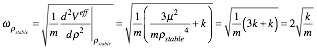
The stability radius for circular orbits is found where force or V^eff derivative is zero.

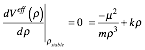(5.2.6a) . (5.2.6b)

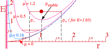
Fig. 5.2.1 Harmonic oscillator effective potentials for angular momenta m=0, 0.12, 0.6, and 1.2.

The frequency for radial oscillation around a circular orbit is a root of 2^nd V^eff-derivative over inertia m.

(5.2.7)

Angular velocity at circular orbit radius relates to angular momentum m=m. (Recall (3.13.4c).)

(5.2.8)

This shows that radial oscillation is twice the angular one so, at least for small oscillations, the path is like the nr :nf =2:1 path in Fig. 3.13.1. In fact, it is an ellipse like the one in Fig. 5.2.2 as described in Sec. 1.5 and Fig. 1.5.1. Now we reprove the elliptic geometry using integrals from (3.13.10a).

(5.2.9)

With constants the solution (5.2.1d) gives

(5.2.10)

We leave it as an exercise to verify the oscillator equation of radius versus time.

(5.2.11)

This shows radial frequency in (5.2.7) is always wr=2√k/m. It seems strange that adding arbitrary amount of a 1/r2 barrier potential to a harmonic r2 potential exactly doubles its harmonic frequency while that frequency is still harmonic, that is, independent of energy. However, it is r2-oscillation, not r-oscillation that is sinusoidal in effective potential Ar2 + B/r2 of (5.2.3). Speed is high at perigee as r bounces off the centrifugal barrier then slows approaching apogee to conserve angular momentum m by Kepler's law.

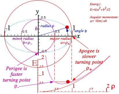
Fig. 5.2.2 Harmonic oscillator effective potential and elliptical orbit turning points

A polar equation of an ellipse of major and minor radii a and b centered at origin as in Fig. 5.2.2 is

. (5.2.12)

Turning points (5.2.5) are r₊=a at angle fa = 0 and r_-=b at fb = π/2. (Check (5.2.5) and (5.2.10)!)

b. Coulomb effective potential

Coulomb effective potentials are plotted for m=1, k=1 in Fig. 5.2.3. Note attractive (–k/r) field has k>0.

(5.2.13)

The four curves are for values of angular momentum: L=m=0, 0.4, 0.5, 0.85, and 2.9. A particle is oscillating in the m=0.85 effective potential with energy E= -0.65. The "real" potential -k/r acts alone for m=0, only.

The turning points for the apogee (r+) and perigee (r-) are drawn for the m=0.85 curve at energy E=-0.65. Again, these points are found by solving for zero KE or where total E=V^eff.

(5.2.14)

(5.2.15a) (5.2.15b)

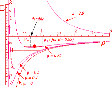
Fig. 5.2.3 Coulomb effective potentials for angular momenta m=0, 0.4, 0.5, 0.85, and 2.9.

Again, the stability radius for circular orbits is found where force or V^eff derivative is zero.

(5.2.16a) (5.2.16b)

Again, frequency for radial oscillation around a circular orbit is a root of a 2^nd V^eff-derivative over inertia.

(5.2.17)

Angular velocityat gives angular momentum m=msois unit ratio nr:nf =1:1.

(5.2.18)

Integral (3.13.10) gives f(r) using (5.2.1) and constants:.

(5.2.19)

The solution (5.2.1d) is a conic section (ellipse, parabola, hyperbola) of radii a and b, as will be shown.

(5.2.20a) (5.2.20b)

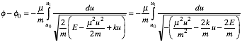
(5.2.20) may be an ellipse with focus at origin as in Fig. 5.2.4. It may also be a hyperbola or parabola depending on whether constant k and E values allow it to escape to infinity, but m is irrelevant for that.

As was the case for the oscillator in Fig. 5.2.2, Kepler's law demands high speed for low r and vice-versa. In Fig. 5.2.2 the trajectory "gallops" very rapidly past the perigee and ricochets off a steeper centrifugal barrier than that of the oscillator. Here the effective potential V^eff(r) slope at the apogee is much gentler than at the perigee, and the perigee generally gets closer to origin than it does for the oscillator.

Fig. 5.2.4 Coulomb V(r)=k/r and orbit ellipse turning points of V^eff(r). (k=1, m=1, m=0.5, E=-0.875 )

c. Geometry of conic section orbits

To clearly understand conic-section orbits, particularly Coulomb orbits, it helps to review their basic geometry. Two fundamental parameters that define all conic-sections are the eccentricity e and the latus-rectum l. Other parameters like major radius a or minor radius b may be derived from e and l.

Fig. 5.2.5 labels (e,l) parameters. The eccentricity e is the ratio between the radial distance r to a point P on the conic and the distance DP= r/e of that point to a vertical line called the directrix DD'. The latus rectum or lat-radius l is the vertical intercept of the conic above the origin quite like the parabolic l defined in Fig. 1.4.3 of Unit 1, and so the l-intercept point must be l/e from the directrix. Horizontal length l/e plus radial X-projection r cos f equals the length r/e of line DP. Polar conic r(f) equations result.

r/e = l/e + r cos f (5.2.21a) r = l + r e cos f (5.2.21b) (5.2.21c)

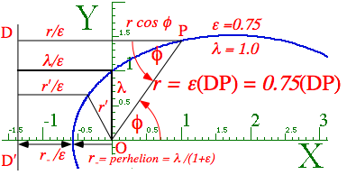
Fig. 5.2.5 Universal definition of conic-section ellipse, parabola, hyperbola (or circle for e=0).

This is a universal conic equation describing all conics and all the purely Coulomb orbits. Note the horizontal intercept or minimum perihelion radius r- occurs at polar angle f=π in Fig. 5.2.5.

perihelion radius = r- = l/(1+e) (5.2.21d)

For zero polar angle f=0 is the max or aphelion radius r+. (Recall that prefix “ap” means “up” in radius.)

aphelion radius = r+ = l/(1-e) (5.2.21e)

As the eccentricity approaches unity (), aphelion radius r+ approaches infinity. The special case (e =1) is called a parabola. For e>1, the (+)-branch of a hyperbola shows up with r+ on the negative axis. The hyperbola is like a BIG ellipse wrapped-around the universe as we try to show in Fig. 5.2.6 below.

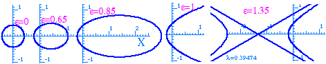
Fig. 5.2.6 Fixed-levolution from circle (e=0)to ellipse (e<1)through parabola (e=1)to hyperbola (e>1)

The parabola is very special, a set with no measure. There are no perfectly parabolic orbits, only some (actually a lot!) that are nearly parabolic. (One example is the path of your pencil if you throw it.)

All the orbits except the perfect parabola (e =1) have a center of symmetry. All orbits except the circle (e =0) have a pair of distinct focal points; one at origin called the prime focus, and another called the secondary focus on the opposite side of the center of symmetry. Universal conic equations favor one focus as “prime” and seem lop-sided. Cartesian equations of conics seem more balanced. (Recall (1.5.7).)

(5.2.22a)

This is invariant to x-y reflections about a center of symmetry (xc, yc) where it has bilateral symmetry.

(5.2.22b)

The harmonic oscillator orbit symmetry center of force is origin (xc, yc)=(0, 0) as in Fig. 5.2.2, but the Coulomb orbits (Fig. 5.2.4) are off the center of force. To understand the orbit equations we need to account for their intrinsic bilateral symmetry: all conics (except zero-measure parabolas) really have two radii (r, r'), two foci (F, F'), two directrix lines (D, D'), and two latus-rectii (or radii) (l, l') as shown in Fig. 5.2.7.

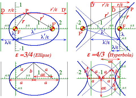
Fig. 5.2.7 Geometry and parameters of conic-sections in polar and Cartesian coordinates

Orbit size and shape are fixed by the sum and difference of the aphelion and perihelion radii (5.2.21d-e).

2a=|r₊+r_-|= |l/(1-e)+l/(1+e)|=|2l/(1-e2)| (5.2.23a) FF' =|r₊-r-|=|l/(1-e)-l/(1+e)|=|2le/(1-e2)|=2ae (5.2.23b)

This is major axis 2a and inter-focal distance 2ae drawn in Fig. 5.2.7 above and Fig. 5.2.8 below.

Let us rectify Cartesian equations (5.2.22a) of conics, for which hyperbolas and ellipses are obviously different animals, with polar equation (5.2.21) that better shows the similarity of ellipse and hyperbola. The latter use l and e while the former use major or minor radii a and b for parameters. A study of the two on the top and bottom of Fig. 5.2.7 lets us learn a great deal about orbital mechanics. We now compare the differences between ellipse and hyperbola in Fig. 5.2.7.The inter-directrix distance DD' is listed below for the ellipse and for the hyperbola. (Here: l'2- l2=(2ae)2 holds for both.)

DD'= r'/e + r/e = l'/e+ l/e DD'= r'/e - r/e =l'/e - l/e

(5.2.24a)ellipse (5.2.24a)hyperb.

The lower Fig. 5.2.7 shows the relation between the two focal radii. For the ellipse the focal radii maintain a constant sum, but the hyperbola maintains a constant difference between radii.

eDD'= r + r' = l + l' = 2a, eDD'= r' - r = = l' - l = 2a.

(5.2.24b)ellipse (5.2.24b)hyperb.

For either case the constant is the major axis 2a of the conic. To see this we check the perigee or apogee of the conic and a point mid-way between. An ellipse’s mid-way point is the top of its semi-major axis b where clearly the focal sum is 2a. But for the hyperbola the mid-way point is more difficult to see since it is “half-way” to infinity (apogee is at ∞ for hyperbolas) as indicated by blue F∞ and F¢∞ lines ending with ∞-symbols in Fig. 5.2.8 below. But, their length difference F∞-F¢∞ (the red-arrow segment) is 2a.

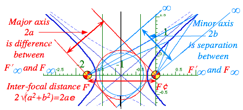
Fig. 5.2.8 Geometry and parameters of hyperbola in tilted 2a-by-2b Cartesian coordinates

The Cartesian coordinate description is based on a rectangular 2a-by-2b box. The 2b sides of this box have slope b/a and are asymptotes of the hyperbola to which it approaches at ∞ as seen in Fig. 5.2.7-8. An ellipse’s 2a-by-2b box has zero slope and holds the whole curve circumscribed within it. In either case the major diameter 2a is the distance nose-to-nose between X-axis intercepts (roots) of ellipse or hyperbola. The minor diameter 2b of the ellipse is the distance side-to-side between Y-axis intercepts of ellipse or of the conjugate branches x²/a²- x²/b² =-1 of the hyperbola (dashed curves) that share the same asymptotes.

In hyperbolic Fig. 5.2.8 the 2a-by-2b box is tilted so it lines up with the asymptote that goes toward ∞ in the upper right or first quadrant. Another such box lines up with the other asymptote of slope -b/a. A difficult part of this "marriage" of Cartesian-based and polar-based descriptions is being able to see the relations in Fig. 5.2.7 tipped over so they line up with an asymptote as in Fig. 5.2.8. We use this to study Rutherford scattering.

To help see line ratios, radii, and axes consider Fig. 5.2.9 that is an abstraction of Fig. 5.2.7 and 8.

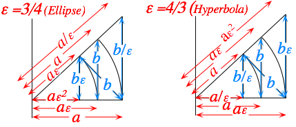
Fig. 5.2.9 Geometric ratio series of parameters for ellipse and hyperbola.

Each successive line segment, tilted or untilted, has a geometrical ratio with its neighbors by a factor e or 1/e. The hyperbolic segments differ from the elliptic ones by replacing the ratio e by 1/e. The relation between a, b, e, and l comes out fairly easily from these diagrams.

For the elliptic geometry (e <1): For hyperbolic geometry(e >1):

b2 = a2 - a2e2 = al , b2 = a2e2 - a2 = al,

b = a √(1-e2 )= √(al), b = a √(e2-1)= √(al).

(5.2.25a)ellipse (5.2.25a)hyperb.

The (l,e)-(a,b) expressions and their inverses follow using (5.2.23).

a = l/(1-e2) a = l/(e2-1)

b2 = l2/(1-e2) b2 = l2/(e2-1)

l = a(1-e2) = b2/a l = a(e2-1) = b2/a

e2 = 1- b2/ a2 e2 = 1+b2/ a2

(5.2.25b)ellipse (5.2.25b)hyperb.

d. Physical and geometrical parameters of Coulomb orbits

A quick way to relate conic geometrical parameters (a and b or e and l) to Coulomb orbital parameters (energy E and angular momentum m) is to equate the perihelion-aphelion radial sums and differences from (5.2.23), that is,

2a =| r+ + r-| = |2l/(1-e2)|, and FF' =| r+ - r-|= |2le/(1-e2)| = 2ae ,

with turning point roots (5.2.15a) . The sum of the roots is diameter 2a.

. (5.2.26)

If one learns just one thing about Coulomb orbits, it is this: the major axis 2a of any orbit is proportional to the Coulomb constant k and the inverse of total energy. Stated another way: Magnitude E of the total orbit energy equals the magnitude |V(2a)|=|k/2a| of potential energy at distance of the orbit's major diameter 2a.

(5.2.27)

Energy with correct sign can be given by separate equations for elliptic and hyperbolic orbits.

(5.2.28a)ellipse (5.2.28a)hyperbola

One extreme case is a perfectly parabolic orbit that has exactly zero total energy and an infinite value for major axis 2a. (E=T+V=0 and a=∞.) Another extreme case is the perfectly circular orbit (r+=r-=a=R=l) for which we see the total energy is exactly half as negative as the potential energy.

(5.2.28b)circle

In other words, the energy needed to achieve a circular orbit starting at radius R, equals one half the energy needed to escape to r =∞ from that point r =R. This is shown by Fig. 5.2.10.

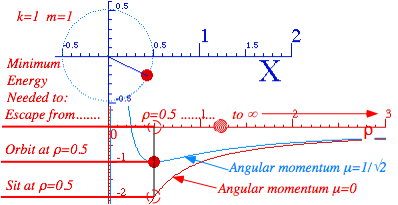
Fig. 5.2.10 Three Coulomb threshold energies: to sit (E=-2), to orbit (E=-1), and to escape (E=0) from R.

A 4^th energy (E=-3) is for sitting at the center (r =0) of a uniform mass planet of radius r =R.

You may recall from discussion of (1.4.18) in Unit 1 and Fig. 1.4.12 that the circular R-orbit energy is one third of the energy needed to escape from sitting dead center (r=0) in a uniform planet of radius R.

To obtain the other geometric parameters we consider the difference of turning points.

(5.2.29)

Solving with 5.2.26 gives eccentricity e and latus-radius l. The latter depends on m=l but not E.

(5.2.30a)

The Cartesian major and minor axes then follow from (5.2.25b)

(5.2.30b)

Below is a summary of the parameter relations that compares Cartesian and polar coordinate views.

Cartesian parameters provide a one-to-one relation between major axis a and energy E, while polar parameters provide a one-to-one relation between latus-radius l and angular momentum m=l.

e. "Diving" orbits

The ratio l/a of latus-radius to major axis or the square of the minor-major axis ratio b/a is

(5.2.31)

"Skinny" orbits with low l/a are called diving or cometary orbits because, like Halley's comet, they dive through the low radius region very quickly and spend most of their time at large r. They have eccentricity near unity (e1), that is, they are nearly parabolic. Near-parabolic orbits must either have low energy (E0), or low angular momentum squared (m2=l20), or both. The extreme case is (m2=l2=0), which is called an s-orbital in atomic physics. Only electrons in s-orbitals have no centrifugal barrier and can "dive in" to interact with the nuclear spins and give rise to Fermi-contact hyperfine energy.

The orbit solution (5.2.20) and the conic equation (5.2.21) are rearranged to give

. (5.2.32a)

This is consistent with the parameter relations (5.2.30). Diving orbits are approximated by

. (5.2.32b)

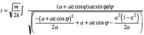
f. Kepler equation of time

Throughout the history of astronomy a most important consideration was the timing of orbits. The time integral (3.13.5b) is rewritten here.

Using conic parameters (5.2.30) for elliptic orbits it becomes

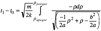. (5.2.33)

For attractive (k>0) potential the r-term in the radical is positive. For elliptic orbits ( E<0) the r2 term is negative. A negative differential (-dr) is used if integral goes from "up" (apogee) to "down" (perigee).

An elegant treatment of the integral uses a new kind of coordinate; the eccentric anomaly coordinate j. Eccentric anomaly j is a polar angle measured from orbit center of symmetry as shown in Fig. 5.2.11.

(5.2.34)

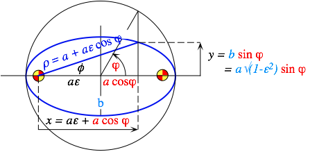
Fig. 5.2.11 Relating eccentric anomaly coordinate j to polar coordinates (r,f).

j is like the harmonic oscillator orbit polar angle except it points at a projection on the a-circle. The use of j simplifies the time integral (5.2.33).

This reduces to the following and expressed in terms of an averaged eccentric angular velocity

(5.2.35a)

(5.2.35b)

This is known as Kepler's Equation of Time. The eccentric velocity is constant only for circular (e=0)orbits. The 3/2-power law (5.2.35b) for orbital period is also derived by Kepler's area rule (3.13.7) (T=2mA/m ). Area of an ellipse (A=πab) and the conic parameter relations (5.2.30) (b2 = al = a m2/km) are used.

T= 2m πab/m = 2m πa√(la)/m = 2m πa3/2√(m2/km)/m= 2πa3/2√(m/k) (5.2.35c)

This agrees with (5.2.35b). Note the connection between energy and time here. All orbits with the same energy have the same period. Having different angular momentum does not affect the frequency of orbit.

5.3 Hyperbolic Orbits in Coulomb Potentials

Two cases of orbits for a Coulomb field have not been considered yet. These are the repulsive potentials with a negative force constant (k-k) and the case with positive energy (E>0) in an attractive potential. Both these involve hyperbolic orbits.

a. Rutherford scattering

Probably, the classical problem of the greatest historical significance to atomic physics is the Rutherford scattering effect involving an alpha or He++ ion of mass m=4 amu. scattering off a gold (Au) nucleus of mass M= 197 amu. and charge q=+97e. Coulomb orbital mechanics is assumed valid until the two nuclei actually "touch", that is, engage their short-range nuclear forces which are much stronger than Coulomb electrostatic fields. The surprising result shown by Rutherford was that the nuclear forces are confined to an incredibly small volume that can only be penetrated by very high energy a-particles. To apply the Coulomb orbit mechanics one neglects the scattering of the a-particle from the atomic electrons which are several thousand times less massive and mostly absent from the region where most of the scattering mechanics actually take place. (Diving orbits spend very little time at small radii.)

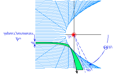
Suppose that a beam of a-particles is sent parallel to the x-axis as indicated by the dashed lines in Fig. 5.3.1a. Without the Gold nucleus at O they would each travel along their parallel lines at constant speed forever. The figure shows how to construct the orbit caused by the Au at O of an a-particle given its energy E and its distance b perpendicular to the beam from the "dead-on" path that would have gone through O had there been no repulsive force. This distance b is called the particle's impact parameter. (See Fig. 5.3.1b.)

The beam energy E sets the major axis 2a = k/E for all the particles in the beam according to (5.2.26). This gives the closest approach point r- = 2a shown in Fig. 5.3.1a where a "dead-on" a-particle aimed right at O would come to a dead stop before reversing its straight-in path to go straight-out.

From Fig. 5.2.8 it is seen that a circle of diameter 2a must be tangent to an axis drawn through the focus perpendicular to an asymptote. The construction in Fig. 5.3.1b takes the beam direction to be the asymptote and the y-axis to be the perpendicular tangent. The line CC' in Fig. 5.3.1a intersects the desired beam impact line at point C, at distance b above the x-axis. About this point a circle of radius a is drawn in Fig. 5.3.1b.

In Fig. 5.3.1b-d the line OCF drawn through the focus O and circle center C contains the second focus O', too. OCF is the orbit symmetry axis (the x-axis in Fig. 5.2.8), so the outgoing asymptote is found by copying the incoming angle BCF to make angle B'CF and outgoing asymptote CB', as shown if Fig. 5.3.1c-d. The polar angle of CB' is the scattering angle Q. The center point C is the orbit center of symmetry about which the dashed focal circle through foci O and O' is drawn in Fig. 5.3.1d. From O and O' the (a,b)-hyperbolic orbit is constructed.

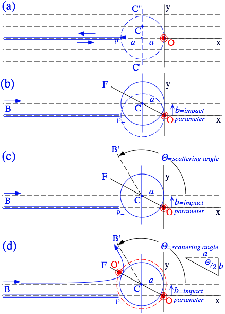
Fig. 5.3.1 Geometrical construction of Rutherford scattering angle and orbit.

A family of Rutherford orbits constant E and variable b is shown in Fig. 5.3.2.

Fig. 5.3.2 Family of iso-energetic Rutherford scattering orbits with varying impact parameter.

Every particle that comes in with impact parameter between b and b+db will go out on an asymptote that has a polar angle between Q and Q-dQ. This is indicated in the Fig. 5.3.2. The asymptotes are displaced slightly and do not point exactly at the nucleus, but as the scattered particle flies farther and farther away, this shift appears negligible. Symmetry about the x-axis (scattering theorists would call that the z-axis) means the azimuth angle about the axis remains constant. So a particle that enters an incremental window =b db perpendicular to beam axis at x=-∞ will be scattered to an area

on a sphere at R=+∞ where is called the incremental solid angle dW. The ratio

(5.3.1)

is called the differential scattering crossection (DSC). The construction in Fig. 5.3.1d gives a formula relating impact parameter and scattering angle.

(5.3.2)

Combining gives the Rutherford DSC.

(5.3.3)

Multiplying the DSC by the input flux density of S particles per (m2sec) at b and the output solid angle dW gives the output particle number S per second in the solid angle dW.

Integrating the DSC over a range of scattering angles gives a partial scattering crossection.

(5.3.4)

A integral over whole sphere from to is the total crossection s. For Rutherford scattering s is infinite; the Coulomb field has an infinitely large "shadow." The boundary of the shadow region, such as is visible in Fig. 5.3.1, is called a caustic or envelope. Later, we shall discuss the calculation of trajectory envelopes, but you should be able to derive the equation for the Rutherford envelope using conic geometry alone. (See exercises.)

The Rutherford caustic has some very big cousins; the interplanetary "bow-waves" of our Sun cruising through the intergalactic Hydrogen. The solar wind varies as 1/r2 so it is effectively a repulsive Coulomb force which may easily exceed the attractive solar gravity. The bow waves are numerous and complex since the effective Coulomb constant k depends on the optical crossection of Hydrogen which in turn depends strongly on solar spectral intensity near various Hydrogen resonances which themselves depend on Coulomb energetics. It is a very Coulombic problem!

b. Hyperbolic equation of time

The equation of time for a hyperbolic trajectory is very different from that of an elliptic orbit. First of all, the orbit period is undefined or infinite. Kepler's law gives the time to go from the perigee point A at r- = a + ae in Fig. 5.3.3 to point P on a Rutherford hyperbola.

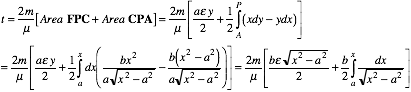
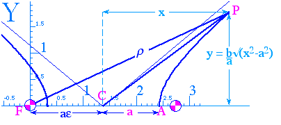
Fig. 5.3.3 Area FPAswept by Rutherford scattering orbit. Area FPA = area FPC+ area CPA

The integral reduces to an inverse hyperbolic or logarithmic function of x.

(5.3.5a)

If it were not for the logarithmic term, the relation between t and x would approach a linear one as x becomes much larger than a. When the particle is closest to the repulsive force center, it is going at the slowest speed it will have on its entire hyperbolic path. After passing the perigee it begins gaining its original speed back again. Since angular momentum is m=mv(∞)b, the x-velocity approaches vx(∞)=v(∞)/e = m/(me b). So we might expect the time distance relation to approach x = vx(∞)t, or

(for x>>a). (wrong!)

Instead, it approaches linear-plus-logarithm.

(for x>>a) (5.3.5b)

This is because it takes so long for the particle m to gain back its initial speed v(∞) that it falls logarithmically behind the distance v(∞)t it might have achieved if it gotten its speed back sooner.

x = v(∞)t - ln(2x/a)/e

The Coulomb potential is called a long range potential because of this. It is forever adding just a little more of the promised velocity like a terribly miserly employer who hoards the pension until it's too late!

Similar effects occur for attractive Coulomb forces. The left branch of the hyperbola in Fig. 5.3.3 is an orbit that would result if the force from point F were attractive, but the particle had positive energy (E>0 above escape velocity). When the particle passes its perigee at its minimum radius r- = ae - a , it is going at the highest speed it will achieve during its entire trajectory. After passing the perigee, the attractive force begins reducing the particle's outward speed a little bit at a time forever and ever. In this case the particle runs logarithmically ahead of where it would be if it had been brought more quickly back to its original speed v(∞) .

5.4. Unified Geometric Development of Coulomb Orbits

The exceptional symmetry properties of the Coulomb potential lend it to extraordinarily simple geometrical constructions of general families of orbits and phase space trajectories. Someone skilled in using a ruler and compass can often out-perform modern computers when it comes to making semi-quantitative predictions and discovering new effects.

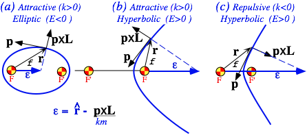
a. The eccentricity vector

For all central force fields of the form

(5.4.1)

there is a guaranteed conservation of the angular momentum vector L defined by

. (5.4.2)

This is easily proved.

. (5.4.3)

The Coulomb field is a special central force (Again, let k>0 be attractive.)

(5.4.4)

This also guarantees conservation of the eccentricity vector e defined by

(5.4.5a)

To show this we consider the following time derivative using (5.4.1-2).

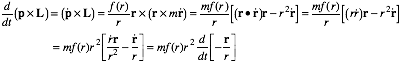
For f(r) = -k/r2 this simplifies and proves the following

(5.4.5b)

where A = km e , known as the Laplace-Hamilton-Gibbs-Runge-Lenz vector, is seen to be a constant in a Coulomb field, as is the eccentricity vector e=A/km , which is proportional to A.

While the A-vector has symmetry group applications, the dimensionless e-vector is more suited for geometrical interpretation. Consider the dot product of e with a radial vector r.

(5.4.6)

This simplifies to the conic equation (5.2.32a) for angular momentum m=L,

(5.4.7)

where the polar angle f is the angle between e and the radial vector r, as shown in Fig. 5.4.1.

Fig. 5.4.1 Eccentricity vector e for the three kinds of Coulomb orbits.

The e-vector can be used to give a simple three-step construction of a general Coulomb orbit for arbitrary initial conditions r=r(0) and p=p(0). The first step shown in Fig. 5.4.2a involves copying the initial launch angle g onto the opposite side of the initial momentum vector p at the launch point r.

The two circles shown in each of Figs. 5.4.2 are first used to copy launch angle SPP' to angle P'PQ. This construction leads to the focus locus. It is not hocus-pocus since we know that foci must reflect to each other from any tangent of a conic with the angle of incidence equal to the angle of reflection.

Then the two circles are used to copy the double angle SPQ below on the opposite side of the initial position vector r to make angle SPT as shown in Fig. 5.4.2b. The line PTR drawn through the construction points P and T will be the energy ratio (R-scale) axis where R is the initial ratio of KE to PE.

(5.4.8)

This R-axis is just the pxL direction and therefore perpendicular to the initial p and tangent PP'.

The final steps are to locate the e -vector on the R-scale (in Fig. 5.4.2c we chose R=-3/8) and extend it to the focus-locus to give the secondary focus F'. From F , F' and the initial point P the entire orbit is constructed.

Notice that a choice of R=-1 would put the second focus F' at infinity and give a parabolic orbit. If R<-1 then second focus F' reappears on the upper left-hand portion of the focus locus above Q, and this results in a hyperbolic orbit of the form shown in Fig. 5.4.1 b.

All positive values of R>0 will point at a second focus F' in the QP section of the focus-locus and give hyperbolas around F' of the form sketched in Fig. 5.4.1 c.

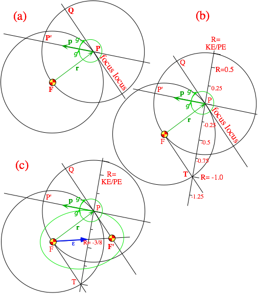
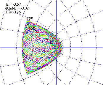
Fig. 5.4.2 Construction of eccentricity vector e and orbit from initial r, p with KE/PE=-3/8.

To prove the construction we write out the eccentricity vector in terms of unit vectors and use (5.4.8).

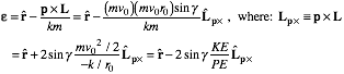(5.4.9)

The unit R-scale distance of 2sin g (in units of r(0)) is thereby justified.

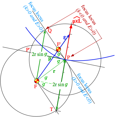
Fig. 5.4.3 Construction of eccentricity vector e and orbit from initial r, p with KE/PE=+1/2.

b. Geometrical derivations

With such a simple construction one can derive some surprising properties of Coulomb orbits and families of orbits like the Rutherford swarm in Fig. 5.3.2.

1. Space bomb

What if a bomb blows up at a certain point r outside of a small planet? An equivalent problem would involve the trajectories of a rarefied electron plasma emitted by a point cathode some distance away from a positively charged sphere or point. What does the particle "cloud" do?

Let us suppose for the sake of simplicity that all the orbiting particles have the same initial speed or energy. Isoenergetic trajectories thrown in all directions will each have one thing in common: each major axis 2a=k/E will be the same for all. This confines their second focus to a circular "focus-locus" of radius PF'= 2a-r around launch point P as shown in Fig. 5.4.4 a.

Each focus F' on the circular focus-locus gives one elliptical orbit. Along the orbit in Fig. 5.4.4 a are a series of time points T, T' , T". The first of these, point T, is special since its second focal radius F'T is colinear with the line F'P from the second focus to the launch point P. This T-point is called a contact point since it is the only point on this particular orbit to contact the envelope or caustic of all the orbits. The shape of the caustic is derived by examining its contacts.

Because all the pairs of focal radii sum to 2a, the following sums are true;

FP + PF' = r + PF'= 2a , and: FT + TF' = 2a .

This implies that sum of the radii from F to T and from T to F' and from F' to P is the following.

FT + TF' + F'P= 2a + F'P = 2a + 2a - r = 4a - r

Furthermore, this is true of all the orbits, so the locus of all their contact points is an ellipse built on the first focus F and the launch point P as a second focus with radii satisfying the following sum.

FT + TP = 4a - r (5.4.10)

This enveloping ellipse is drawn in Fig. 5.4.4 b and clearly visible as the enveloping boundary in Fig. 5.4.4 c. The actual 3-dimensional envelope is surface of revolution or prolate ellipsoid around the FP axis. There is one "diving orbit" that reaches a height of 2a - r above P before falling back to the center of force F. (If it survives that it would be a miracle!)

Notice that every point r inside the elliptical caustic boundary in Fig. 5.4.4 c has two trajectories passing through it, while the points on the boundary have only the one contacting trajectory and a dense set of "near misses." This structure is a "natural" coordinate system with the launch point P and the force center F being point singularities. The launch point has an infinite number of trajectories passing through it. By launching a projectile from point P with fixed energy (ratio R=-3/8, here) there are two ways you can hit a general inside point r. (Actually, there are four ways counting going forwards and backwards.) Can you show how to construct these hits?

Another interesting geometrical question: after the bomb explodes or you launch multiple projectiles, which (if any) of the orbits first returns its particle to the initial launch point P ?

Fig. 5.4.4 Construction of orbital caustic envelope of orbits with KE/PE=-3/8.

2. Comet tails (and heads)

For a repulsive Coulomb potential like the solar wind there are the caustics associated with the shape of an idealized model of a boiling comet. Suppose all the particles that boil off from the sun's heat leave with the same speed and are repelled by the solar wind according to the same Coulomb force. The resulting cloud will make something like what we observe as the beautiful comet "tail." What is the geometry of the ideal comet tail, if we assume the comet itself is moving slowly compared to its streaming ejecta? Two examples are shown below.

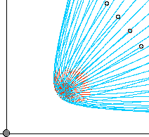
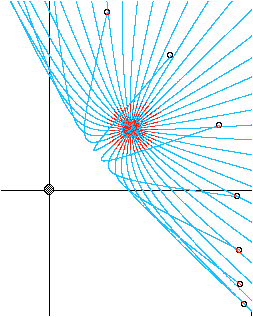
Fig. 5.4.5 Examples of comet-like caustics and trajectories for positive values of KE/PE.

5.5. Coulomb Orbits in Electric Field

Coulomb orbit equations in the presence of a uniform electric field are exactly separable in parabolic coordinates. This leads to an exact analytic solution in terms of quadrature integrals for the classical Stark effect. This begins with the discussion after (3.14.14) in Unit 3.

a. Parabolic coordinates

As before, orbital motion lies in the xy-plane but now has a fixed uniform electric or other force acting in the x-direction. The following (u,v) to (x,y) coordinate transformation is useful.

(5.5.1a)

Squaring and summing gives the polar radius in terms of either coordinate set.

(5.5.1b)

Together the two equations involving u2 and v2 are solved to give the inverse transformation.

(5.5.1c)

Rewriting (5.5.1bc) gives equations for pairs of confocal parabolas shown in Fig. 5.5.1.

(5.5.1d)

The translation u2/2 of the u=const. parabola is also its focal distance and similarly for v=const.

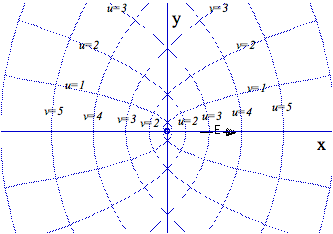
Fig. 5.5.1 Confocal parabolic coordinates

The Jacobian transformation matrices are as follows.

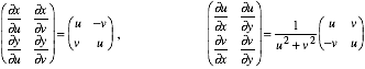(5.5.2)

This leads to a diagonal covariant and contravariant metric tensor. (This is an OCC system.)

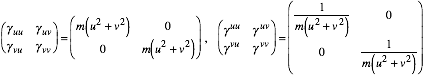
(5.5.3)

The resulting Hamiltonian is as follows in Cartesian coordinates.

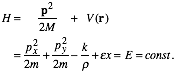(5.5.4)

In parabolic coordinates it becomes separable.

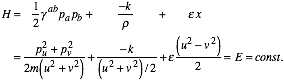(5.5.5a)

However, we must define a "pseudo-Hamiltonian" .

(5.5.5b)

This separates cleanly into two independent parts.

(5.5.5b)

The parts must therefore each be constant and the constants must sum to zero.

(5.5.5b) (5.5.5b)

The effective potentials are quadratic and quartic combinations that depend on energy E in an unusual way while the constant h together with Coulomb constant k play the role of pseudo-energies. As usual, the motion is a stable bound state only for negative total energy E=-|E|.

However, an electric field potential eventually falls below any bound state energy however negative and stable it might have been. Larger E-field potential gradient e makes it happen sooner as seen in Fig. 5.5.2 below. In Fig. 5.5.2(a) the v-turning points are quite close and stable for a small field e=1. However, for a larger field e=2 they have moved away from origin and are on the threshold of disappearing altogether. The v-motion for Fig. 5.5.2(b) is about to blow up.

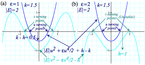
Fig. 5.5.2 Effective potentials for parabolic coordinates

When v-motion blows up and u-motion is stable, the particle will fly out between u=const. curves in Fig. 5.5.1 without u changing much. That is, it will follow a nearly parabolic trajectory that resembles closely that of a particle falling in a uniform gravitational field. For positive field (e>0) the parabola opens to the left which is the negative potential or "down-field" region. For negative field (e<0) the parabola opens to the right and the u-coordinate is the one that is capable of blowing up while v remains stable.

For sufficiently small fields, as in Fig. 5.5.2(a), both the u and v motions are stable and independent oscillation takes place between them. Both motions are highly anharmonic, but they are bounded by the parabolic coordinate lines in all such cases, as seen in Fig. 5.5.3. Surprisingly, the oscillations can take place equally on either the "down-field" side as in Fig. 5.5.3(a), the center as in Fig. 5.5.3(b), or on the "up-field" side.

The time dependence of such a system is a little tricky since it is governed by a "pseudo-Hamiltonian" (5.5.5b). An example of a "pseudo-Hamiltonian" equation is as follows.

(5.5.6)

where defines a pseudo-time that gets finer and finer scale as radius r increases.

(a)

(b)

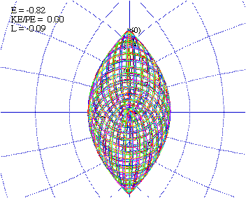
Fig. 5.5.3 Examples of bound-state motion restricted by parabolic coordinates

References

Unit 5 Problems

Repulsive oscillation

5.2.1 Derive formulas for the orbital path of a mass m in an isotropic repulsive quadratic potential

(k>0)

Discuss any analytic or geometric properties of the resulting orbits.

Attractive oscillation

5.2.2 Verify (or correct) the oscillator equation of time in (5.2.11). Verify turning point formulas in terms of a orbit radii a and b.

Coulomb approach-avoidance

5.2.3 (a) Derive an equation of time for the attractive Coulomb potential

(k>0)

(b) Do the same for a repulsive potential (k<0) and discuss how it differs from (a).

Dyin' Ion

5.2.4 Suppose an ion of mass m is orbiting a heavy atom of mass M>>m (Assume M fixed) which is polarized by the ion so it has a dipole moment p=aE that always points along the line connecting the two particles. ( Let E be the Coulomb field at the atom due to the ion of charge q. Let polarizability a be constant.)

(a) Derive the force and potential power laws for the ion.

(b) Discuss the stability radii, turning points, and oscillation frequencies (if any exist.)

(d) Try to derive an equation of time.

Rutherford Coulomb

5.3.1. Use geometry to derive the equation of the Rutherford scattering caustic (contacting envelope) as a function of alpha particle mass m, Coulomb constant k and beam energy E.

(a) How many eV of energy are needed to get an a⁺⁴ particle onto the Au⁺⁷⁹ nuclear surface at r= 1fm?

Rutherford Hard-ball

5.3.2. Consider a beam of iso-energetic particles scattering elastically from a hard sphere of radius R.

(a) Derive the relation between scattering angle and impact parameter.

(b) Derive the differential scattering crossection and (if possible) the total crossection. Discuss your results and compare to Coulomb scattering.

Rutherford Spring-time

5.3.3. Consider an attractive isotropic harmonic oscillator potential (3.14.2) with a mass m particle orbiting.

(a) Derive the relations between the elliptical orbit axes and the orbit energy and angular momentum.

(b) Derive the shape of the contacting envelope or caustic for a "space-bomb" that expels isoenergetic particles at a point some distance from the force center.

Two burns

5.3.4. Space shuttle is in circular orbit of radius R₀ and in two burns moves to circular orbit of radius nR₀.

(a) Describe or sketch (for n=2 and 3) the quickest way to do this.

(b) Compute energy and angular momentum of each stage in terms of original energy E₀ and momentum m_o.

Momentum Around

5.3.5. A construction was given for the position vector trajectory r(f) in a Coulomb potential by constructing the eccentricity vector e. These paths were circles, ellipses, parabolas, and hyperbolas.

(a) Describe how to extend the e-vector construction to also construct momentum p-paths in phase space. Do an example for R=KE/PE = -3/8 and g= 30°.

(Hint: Get the r-paths first. Then consider vectors L= rxp and exL. Be creative! You may use the programs to find what kinds of paths p can make.)

Optimum range angle

5.3.6. For plane trajectories in uniform gravity a a=45° launch angle gives maximum range. Also, there is no maximum range (given by effective longitude angle r) for a given angle if you have enough v0. For ballistic missiles traveling in space (or for war on the moon) all is different.

(a) Use geometry to derive the maximum range longitude angle r along the Earth's surface as a function of the launch elevation angle a above the horizon neglecting Earth spin. (First, why is r so limited?)

(b) Use geometry to derive launch angle a which throws a missile to a given range r with minimum energy. Compare result with that of part (a).

Aiming with geometry

5.3.7. For plane trajectories in uniform gravity any point can be hit if you have enough v0. For fixed v0 a given point can be hit with 0, 1, or 2 different trajectories.

(a) How is this situation the same or different for hitting objects in space around a gravitating body? How do you tell whether you can hit a given point.

(b) Assuming you can hit a point use geometry to derive launch angle or angles a which achieve a hit with the given launch energy. Construct an example.